RESOLUTION STATE INTERFACE · EQUATION REFERENCE

RSI Equations

Matthew Tripp Zejda

The ledger, the two gates, and the relations that connect a declared system to its observable readouts.

I develop Resolution State Interface as a scalar, deterministic account of system resolution. I begin by declaring the system and its interface, make the energy ledger explicit, then distinguish what is admitted now from what changes next. Universal Relativity names the requirement that the same underlying account carry across domains rather than change its meanings from one example to another.

The Core-12 remains the central reference. The lettered sections preserve the supplementary equation families and their labels, while the final section separates further source relations from the core numbering. Every expression has a readable transcription, an explanation, and its source location.

RSI Terminology Introduction to Universal Relativity

Find an equation, label, or topic · A–Z

Names and source labels point to the full entries below. Repeated equations retain their distinct source locations.

Find a symbol or notation role

The same letter can have different source-local roles. The equation and its normalization determine the meaning.

S; S_res: Resolution-state admission ratio; the plain-text alias S_res denotes the same gate.
S in S11 fixed point: The local channel-sum symbol in the extended fixed-point treatment, not the admission ratio.
E_A: Anchor budget, with its particular system and normalization declared.
E_F: Field budget, in the same normalization as the other quantities in its equation.
ΣE; SigmaE: Single field-plus-anchor ledger.
ΣE_R: The separately stated shared-field multi-anchor ledger.
T: Energy per recursion layer; specific-energy scale in the separately normalized gravity mapping.
D_E: Dimensionless recursion participation count, not a distance.
D_E,system effective: System-depth readout obtained from matching the same anchor budget.
A_P; AP(r): Declared geometry carrier with the normalization needed by the gate.
C in AP(r): The regime mapping coefficient inside the shell carrier.
C in S11 power law: The local dimensionless amplitude of that strong-coupling helper.
D_c: Change-gate ratio; not a probability.
K: The aggregate engine, not a channel coefficient.
K_ch: A channel coefficient in the engine sum.
K_0: The common-load channel sum, sum(K_ch θ).
B_T: The source-local boundary term; energy or pacing units depend on the stated normalization.
θ; Theta_f: Sign or coherence factor, not a hidden distance law.
Q_i: Partner contribution in the anchor-budget sum.
U_i: Identity contribution in the source tally.
N_C: Strong-domain contact-normalization readout.
R; R_k: Nuclear separation in Equation 11 and its declared strong-domain uses.
μ; ℏc: Resolution scale and conversion factor in S11 scale.
E_F*: Fixed reference energy for the strong-coupling helper family.
α_RSI; α_0; β: Dimensionless strong coupling, its reference value, and the local logarithmic derivative.
b in S11 b fit: Log-law coefficient fixed by the source’s two reference values.
b in α(b); δb: Impact parameter and transverse increment in the optical readout.
σ; w_perp: Line tension and declared effective width in the strong overlay.
Z; δ_k: Fractional resolution contrast and its segment-level readout.
Z_t: Non-core tension helper requiring its own normalization.
Σ_Qθ; α_Q: Partner sum and the scale required by the nucleation matching condition.
f_i; λ_ij: Distinct normalized partner-share and stability-influence readouts.
W_c: Threshold excess D_c − 1 in the overview diagnostic.
r_h; S_ref: Exterior horizon radius and declared reference resolution.

Reading the equations

I use core for the numbered framework relations; supplement or helper for a specified specialization, translation, or readout. An internal derivation, an adopted model form, a calibration, and an independently tested prediction are different kinds of support.

The source’s three claim tiers distinguish derived structure, interpreted overlays, and speculative extensions. Its separate evidence ladder runs from unit and role checks through calibration reuse, cross-domain tests, and stated failure conditions. A tier number is not itself an observation or a validation result.

Equations are shown in mathematical and plain-text form. The optional LaTeX panel provides a standalone transcription using expanded symbol names. The symbols and source labels remain identifiable without loading a script or external mathematics renderer.

R2: §§1.6, 7.4, 15.5; Appendices E–F.

Keep the account and its units fixed

In the main ledger, E_F, E_A, and T are energies, D_E is dimensionless, and A_P includes the mapping that makes S dimensionless. In the gravity calibration, the source also uses energy per reference mass: GM/r has units J/kg. The same printed letter does not make joules and joules per kilogram interchangeable.

The engine has corresponding source-local conventions. In the extended energy-normalized treatment, K and K_ch are dimensionless and B_T has energy units. In the Introduction’s Appendix A pacing convention, K is specific power and B_T is a time, so K B_T is specific energy. Each use of Equation 7 must keep its numerator and denominator in one declared normalization.

Repeated symbols need their local definitions. The extended fixed-point derivation uses S for a channel sum; that is not the admission ratio S = E_A/A_P. The strong power-law amplitude C is not the shell-mapping coefficient C. The source’s reference-energy star E_F* and fixed-point star E_A* are retained where they distinguish those quantities.

Shared equations constrain one another. Equations 3 and 5 imply D_c = D_E when they use the same nonzero account. Consequently, a primitive positive integer D_E does not simultaneously describe a D_c < 1 band under those identical meanings. An effective change budget or system-depth interpretation must be declared; I do not make the constraints disappear by treating coupled quantities as independent controls.

The partner-sum form of Equation 10 and the procedural form of Equation 12 are the Core-12 reference forms. The Introduction’s overview allocation and threshold-excess expressions remain separately identified in section M. These distinctions let the reader follow the sources without treating unlike formulas as synonyms.

R1: §§2.3–2.12; R2: §1.20.5, §15.5, Appendix A.2 and A.7–A.8; R3: pp. 60, 132–133. The D_c = D_E observation is direct substitution in the displayed equations, not a separately named source theorem.

Browse the equation families

A. Core-12
B. Strong-domain helpers · S11
C. Section 4 · Interface and calibration
D. Section 6 · Boundary identities
E. Section 7 · Composite and transfer ledgers
F. Section 8 · Change-gate bands
G. Section 9 · Engine fixed point
H. Section 17 · Transverse contrast
I. Section 18 · Redshift and composition
J. Section 19 · Nuclear shell readout
K. Section 20 · Bounds, pacing, and nucleation
L. Section 21 · Exterior horizon helpers
M. Further source relations

A. Core-12

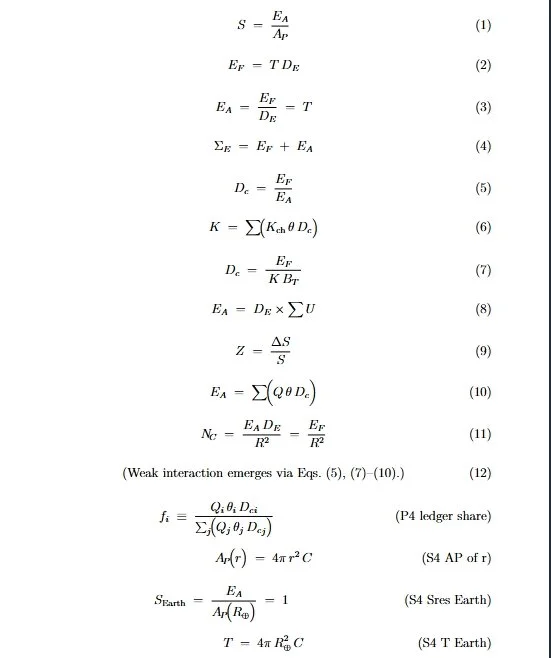
The first four relations establish the ledger. Equations 5–12 then describe change, engine closure, identity accounting, and domain use. Equation 12 is a procedural statement, not a thirteenth independent variable.

Equation 1 · eq:1

Resolution State Law

S=\frac{E_A}{A_P}

Read as: S = E_A / A_P

I begin with the admission question. The anchor budget is evaluated against the declared interface carrier. In the stated threshold convention, S ≥ 1 admits the configuration and S < 1 does not. This is the existence gate, not a force or a probability.

Conditions and scope. A_P must be nonzero and use the same normalization as E_A. In the joule ledger it is a mapped energy carrier, not a bare area in square metres. Admission does not replace the separate change test.

LaTeX transcription

S=\frac{E_A}{A_P}

Source. R1: §2.1 · R2: §§1.10.1, 1.20.5; Appendix A.4

Equation 2 · eq:2

Recursive Field Energy

E_F=T D_E

Read as: E_F = T * D_E

I count the participating recursion layers and multiply by the per-layer budget. T is energy per Resolution State Unit layer; D_E is the dimensionless participation count. Constant T gives a field budget linear in that count.

Conditions and scope. D_E is not radius or distance. A later effective system-depth readout must be declared as such; it is not permission to hide interface geometry inside a layer count.

LaTeX transcription

E_F=T D_E

Source. R1: §2.2 · R2: §2.4; Appendix A.3

Equation 3 · eq:3

Anchor Energy

E_A=\frac{E_F}{D_E}=T

Read as: E_A = E_F / D_E = T

The anchor quantity is the field budget per participating layer. The equality with T follows when the field budget is the one described by Equation 2. At the one-layer boundary, E_F, E_A, and T coincide.

Conditions and scope. The division requires D_E ≠ 0. Applying Equations 3 and 5 to the same nonzero quantities entails D_c = D_E by substitution. I do not treat those coupled quantities as independent inputs.

LaTeX transcription

E_A=\frac{E_F}{D_E}=T

Source. R1: §2.3 · R2: §1.10.3; Appendix A.3

Equation 4 · eq:4

Total Recursive Energy

\Sigma E=E_F+E_A

Read as: SigmaE = E_F + E_A

I keep the field and anchor parts visible in one energy ledger. This is the single-account partition; composite sums and the shared-field multi-anchor convention are listed separately below.

Conditions and scope. Conservation for a closed system additionally requires that the declared boundary exclude unaccounted exchange. A displayed partition alone does not establish that every transfer has been measured or that shared energy has not been counted twice.

LaTeX transcription

\Sigma E=E_F+E_A

Source. R1: §2.4 · R2: §§1.10.4, 2.2

Equation 5 · eq:5

Deterministic Collapse Ratio

D_c=\frac{E_F}{E_A}

Read as: D_c = E_F / E_A

After admission, I compare the field load with the anchor budget. The source classifies values below one as stable, unity as threshold, and values above one as collapse or forced reconfiguration. The engine and available channels supply the transition account.

Conditions and scope. E_A must be nonzero. The ratio is not an event probability or, by itself, a measured lifetime. Using an effective change capacity rather than the original anchor budget requires an explicit declaration.

LaTeX transcription

D_c=\frac{E_F}{E_A}

Source. R1: §2.5 · R2: Appendix A.6

Equation 6 · eq:6

Recursive Engine

K=\sum_{\mathrm{ch}}(K_{\mathrm{ch}}\theta D_c)

Read as: K = sum_ch(K_ch * theta * D_c)

I aggregate the active channel contributions. K_ch sets a channel scale, θ carries the declared sign or coherence factor, and D_c supplies the load. An inactive channel can contribute zero through its orientation factor.

Conditions and scope. K_ch is not the total engine K. The factorization K = K_0 D_c used later requires a common D_c across the summed channels and a specified channel sum. Geometry remains in the carrier rather than in θ.

LaTeX transcription

K=\sum_{\mathrm{ch}}(K_{\mathrm{ch}}\theta D_c)

Source. R1: §2.6 · R2: Appendix A.7

Equation 7 · eq:7

Engine-Regulated Closure

D_c=\frac{E_F}{(K B_T)}

Read as: D_c = E_F / (K * B_T)

The engine-regulated form compares the field quantity with the effective capacity K B_T. Because K itself depends on D_c, a coupled use of Equations 6 and 7 is a closure problem rather than two unrelated substitutions.

Conditions and scope. K B_T must be nonzero and carry the same units as the numerator. The energy-normalized and specific-energy/pacing conventions are distinguished in the normalization note. Equating K B_T with the Equation 5 denominator also requires the same account.

LaTeX transcription

D_c=\frac{E_F}{(K B_T)}

Source. R1: §2.7 · R2: Appendix A.7

Equation 8 · eq:8

Identity Summation

E_A=D_E\sum_i U_i

Read as: E_A = D_E * sum_i(U_i)

I express the declared anchor budget through participating identity contributions. U_i is a contribution to the tally, not an undefined count that can be multiplied into an energy without a mapping.

Conditions and scope. The inventory, depth, and normalization belong to the specified system. Equating this tally with the partner sum of Equation 10 is legitimate only when both describe that same anchor budget.

LaTeX transcription

E_A=D_E\sum_i U_i

Source. R1: §2.8 · R2: §15.5; Appendix A.8.1

Equation 9 · eq:9

Recursive Redshift

Z=\frac{\Delta S}{S}

Read as: Z = Delta(S) / S

I report a fractional resolution-state contrast. In the source-to-observer comparison, the denominator is the source state and ΔS = S_obs − S_source. Positive Z then means the observer readout is larger than the source readout.

Conditions and scope. The reference state must be nonzero and the comparison must use compatible meanings and normalization. Calling this diagnostic redshift does not by itself establish the empirical mapping for every optical or cosmological regime.

LaTeX transcription

Z=\frac{\Delta S}{S}

Source. R1: §2.9 · R2: Appendix A.10

Equation 10 · eq:10

Multi-Body Anchor Closure

E_A=\sum_i(Q_i\theta_i D_{c,i})

Read as: E_A = sum_i(Q_i * theta_i * D_c_i)

I close the anchor budget through the participating partners instead of dividing energy by hand. Each term carries the participant contribution, its sign or coherence factor, and its collapse ratio.

Conditions and scope. This is the budget equation identified by the Core-12 reference, the Introduction’s solver summary, and Appendix A.8. Normalized ledger shares and the overview’s normalized influence allocation are separate readouts, not interchangeable forms of this energy sum.

LaTeX transcription

E_A=\sum_i(Q_i\theta_i D_{c,i})

Source. R1: §2.10 · R2: §15.5, p. 247; Appendix A.8, p. 266

Equation 11 · eq:11

Nuclear Coupling

N_C=\frac{E_A D_E}{R^2}=\frac{E_F}{R^2}

Read as: N_C = (E_A * D_E) / R^2 = E_F / R^2

I use this strong-domain relation for contact normalization. R is the effective nuclear separation handle, and the second form uses E_A D_E = E_F for the same quantities.

Conditions and scope. This is the named exception containing an explicit squared separation outside A_P. It is not a second general existence gate. With energy in joules and R in metres, N_C has units J/m², not newtons without a further length conversion.

LaTeX transcription

N_C=\frac{E_A D_E}{R^2}=\frac{E_F}{R^2}

Source. R1: §2.11 · R2: Appendix A.9 · R3: “Equation 11: Nuclear Coupling,” pp. 91–93

Equation 12 · eq:12

Weak-Domain Closure

Weak interaction emerges via Eq. 5 and Eqs. 7–10; the engine is defined by Eq. 6.

Read as: Weak interaction emerges via Eq. 5 and Eqs. 7–10; the engine is defined by Eq. 6.

I treat weak behavior as emergence through the change gate, engine closure, identity accounting, and partner allocation. The solver-summary wording uses Equation 5 and Equations 7–10; the Core-12 reference describes the collapse loop in Equations 5–7 with Equation 10.

Conditions and scope. This numbered statement introduces no independent algebraic primitive. The overview diagnostic W_c = D_c − 1 is listed separately. Neither the statement nor the diagnostic alone supplies a quantitative decay-rate law.

Source. R1: §2.12 · R2: §15.5, p. 247

B. Strong-domain helpers · S11

These relations translate and specialize the strong-domain account. Their resolution scale, reference energy, fitted coefficients, and finite-window assumptions belong to this helper family; they are not additional Core-12 laws.

S11 scale · eq:S11.scale

Strong-Domain Resolution Scale

\mu=\frac{\hbar c}{R}

Read as: mu = hbar * c / R

This helper translates a declared nuclear separation into the energy-like resolution scale used by the strong-coupling overlay. It connects the R description of Equation 11 to the μ description of the following helpers.

Conditions and scope. R must be positive and the units of ℏc and R must agree. The relation belongs to the strong-domain overlay; it does not redefine recursion depth as a distance.

LaTeX transcription

\mu=\frac{\hbar c}{R}

Source. R3: “Equation 11: Nuclear Coupling,” p. 91

S11 alpha def · eq:S11.alpha.def

Dimensionless Strong Coupling

\alpha_{\mathrm{RSI}}(\mu)=\frac{E_F(\mu)}{E_F^*}

Read as: alpha_RSI(mu) = E_F(mu) / E_F_star

I normalize the scale-dependent field budget by a fixed reference energy E_F*. The quotient gives the coupling used in this family of strong-domain helpers.

Conditions and scope. The reference energy must be nonzero, fixed for the stated mapping, and expressed in the same units as E_F(μ). This coupling is not the deflection angle α(b) used in the optical overlay.

LaTeX transcription

\alpha_{\mathrm{RSI}}(\mu)=\frac{E_F(\mu)}{E_F^*}

Source. R3: “Equation 11: Nuclear Coupling,” p. 91

S11 NC alpha · eq:S11.NC.alpha

Coupling Form of Nuclear Normalization

N_C(R)=\frac{E_F^*}{R^2}\alpha_{\mathrm{RSI}}(\mu=\hbar c/R)

Read as: N_C(R) = (E_F_star / R^2) * alpha_RSI(mu = hbar*c/R)

This is Equation 11 expressed through the reference energy and the dimensionless coupling. The star on E_F identifies the fixed reference scale from S11 alpha def.

Conditions and scope. The formula retains the strong-domain separation factor. It does not introduce an additional radial factor into another core equation or permit independent retuning of the reference energy at every scale.

LaTeX transcription

N_C(R)=\frac{E_F^*}{R^2}\alpha_{\mathrm{RSI}}(\mu=\hbar c/R)

Source. R3: “Equation 11: Nuclear Coupling,” p. 91

S11 alpha log · eq:S11.alpha.log

Logarithmic Coupling Model

\alpha_{\mathrm{RSI}}(\mu)=\frac{\alpha_0}{1+b\ln(\mu/\mu_0)}

Read as: alpha_RSI(mu) = alpha0 / (1 + b * ln(mu/mu0))

The source adopts this one-loop-style logarithmic model as a strong-domain overlay. α_0 is the coupling at the reference scale μ_0, while b is fixed through the declared two-point calibration.

Conditions and scope. This is an adopted modeling form, not a derivation of all strong-interaction dynamics from Equation 11. The scale ratio must be positive and the denominator must remain nonzero in the stated window.

LaTeX transcription

\alpha_{\mathrm{RSI}}(\mu)=\frac{\alpha_0}{1+b\ln(\mu/\mu_0)}

Source. R3: “Equation 11: Nuclear Coupling,” p. 91

S11 beta log · eq:S11.beta.log

Beta Function of the Logarithmic Model

\beta(\alpha)=\frac{d\alpha}{d\ln\mu}=-\frac{b}{\alpha_0}\alpha^2

Read as: beta(alpha) = d(alpha)/d(ln mu) = -(b/alpha0) * alpha^2

Differentiating the stated logarithmic model gives this beta function. Its negative sign for positive b and α_0 expresses weakening with increasing resolution within that model.

Conditions and scope. The derivative inherits the same fixed parameters and permitted scale window. It is a consequence of S11 alpha log, not independent empirical confirmation of the model.

LaTeX transcription

\beta(\alpha)=\frac{d\alpha}{d\ln\mu}=-\frac{b}{\alpha_0}\alpha^2

Source. R3: “Equation 11: Nuclear Coupling,” p. 91

S11 b fit · eq:S11.bfit

Two-Point Calibration of b

b=\frac{\alpha_0/0.118-1}{\ln(M_Z/m_\tau)}\approx0.456

Read as: b = (alpha0/0.118 - 1) / ln(M_Z/m_tau) ≈ 0.456

The source fixes the logarithmic parameter using its stated anchors: (μ_0, α_0) = (m_τ, 0.33) and a coupling of 0.118 at M_Z. The displayed approximation is the value reported for that calibration.

Conditions and scope. These are source calibration choices, not a claim about the latest recommended particle-data averages. The ratio of scales must use compatible units; a new calibration is a separately declared model choice.

LaTeX transcription

b=\frac{\alpha_0/0.118-1}{\ln(M_Z/m_\tau)}\approx0.456

Source. R3: “Equation 11: Nuclear Coupling,” p. 91

S11 sigma · eq:S11.sigma

Planar-to-Line Tension Readout

\sigma\simeq N_C w_\perp

Read as: sigma ≈ N_C * w_perp

I map the strong-domain planar normalization into a line-tension description through the effective corridor width w_perp. This is the source’s route from the nuclear normalization to its confinement comparison.

Conditions and scope. The width is an explicit part of the mapping. J/m² multiplied by metres gives J/m. The approximation is not permission to treat the original N_C quantity as a force without declaring this conversion.

LaTeX transcription

\sigma\simeq N_C w_\perp

Source. R3: “Equation 11: Nuclear Coupling,” p. 92

S11 match · eq:S11.match

Strong-Domain Matching Condition

\frac{E_F^*\alpha_{\mathrm{RSI}}(\mu_t)}{R_t^2}=\frac{\sigma}{w_\perp},\quad\mu_t=\frac{\hbar c}{R_t}

Read as: E_F_star * alpha_RSI(mu_t) / R_t^2 = sigma / w_perp; mu_t = hbar*c/R_t

I impose continuity between the short-distance coupling model and the confinement-side normalization at the declared transition separation R_t. Given one of the reference energy or corridor width, the condition fixes the other.

Conditions and scope. The two sides must represent the same normalization at the same transition. This is a matching prescription with declared inputs, not a separate measurement of every parameter.

LaTeX transcription

\frac{E_F^*\alpha_{\mathrm{RSI}}(\mu_t)}{R_t^2}=\frac{\sigma}{w_\perp},\quad\mu_t=\frac{\hbar c}{R_t}

Source. R3: “Equation 11: Nuclear Coupling,” pp. 91–92

S11 fixed point · eq:S11.fp

Fixed Point with a Local Channel Sum

D_c^2=\frac{E_F}{S B_T}

Read as: D_c^2 = E_F / (S_channel * B_T); here the displayed S is the local channel sum.

In the fixed-point derivation, the local letter S denotes sum(K_ch θ), so K = S D_c. Substitution into Equation 7 gives the squared-ratio relation. I distinguish this local channel-sum usage from the admission ratio S = E_A/A_P.

Conditions and scope. The strong helper by itself does not define a second existence-gate law. The channel-sum reading is explicit in the engine–nucleation derivation; replacing that sum by the admission ratio would require an additional identification not supplied there.

LaTeX transcription

D_c^2=\frac{E_F}{S B_T}

Source. R3: “Equation 11: Nuclear Coupling,” p. 92; “Engine–nucleation scaffold,” Lemma 19.5, p. 132

S11 power law · eq:S11.pow

Finite-Window Power-Law Coupling

\alpha_{\mathrm{RSI}}(\mu)=C(\mu/\mu_0)^{-p}

Read as: alpha_RSI(mu) = C * (mu/mu0)^(-p)

The source presents this finite-window alternative under its stated resolution-thinning and bounded-tension assumptions. C is the amplitude of this coupling model and p is its exponent.

Conditions and scope. This local C is not the mapping coefficient inside the shell carrier A_P(r). The power law remains a scoped supplementary model and is not asserted to replace the logarithmic form over every scale.

LaTeX transcription

\alpha_{\mathrm{RSI}}(\mu)=C(\mu/\mu_0)^{-p}

Source. R3: “Equation 11: Nuclear Coupling,” Lemma 14.1, p. 92

C. Section 4 · Interface and calibration

The repeated core definitions retain their source labels. The shell carrier and Earth-reference relations then make the geometry and normalization explicit. The gravity calibration uses a specific-energy convention, distinguished below from an unnormalized joule ledger.

S4 Sres · eq:S4.SresDef

Section 4 Admission Definition

S=\frac{E_A}{A_P}

Read as: S = E_A / A_P

This section-specific label restates Equation 1 for the gravity-calibration discussion. It keeps the same admission quantity rather than defining a second S.

Conditions and scope. The carrier and anchor budget must be declared in the same normalization before the reference pin is applied.

LaTeX transcription

S=\frac{E_A}{A_P}

Source. R2: §§1.10.1, 15.5; Appendix A.4

S4 SigmaE · eq:S4.SigE

Section 4 Ledger Definition

\Sigma E=E_F+E_A

Read as: SigmaE = E_F + E_A

The gravity-reference discussion retains the same explicit ledger as Equation 4. The local tag is a route back to that section, not another energy reservoir.

Conditions and scope. The accounted boundary still matters. Moving between an energy and a per-reference-mass description requires converting every ledger quantity consistently.

LaTeX transcription

\Sigma E=E_F+E_A

Source. R2: §§1.20.5, 15.5; Appendix A.2

S4 Z · eq:S4.Zdef

Section 4 Shift Definition

Z=\frac{\Delta S}{S}

Read as: Z = Delta(S) / S

This local reference repeats the fractional shift of Equation 9 for the calibration discussion. The source state supplies the denominator in a source-to-observer comparison.

Conditions and scope. A fixed reference and compatible normalization are required; the repeated label is not an additional redshift mechanism.

LaTeX transcription

Z=\frac{\Delta S}{S}

Source. R2: §15.5; Appendix A.10

S4 AP of r · eq:S4.AP.sphere

Spherical Anchor-Plane Carrier

A_P(r)=4\pi r^2 C

Read as: A_P(r) = 4 * pi * r^2 * C

I put the spherical interface geometry and its mapping coefficient inside A_P. At fixed E_A and C, doubling r quadruples the carrier and divides S by four.

Conditions and scope. That is a conditional scaling result. C has units J/m² in the joule ledger, or corresponding specific-energy units per area in the reference-mass convention. A corridor needs its own declared effective carrier.

LaTeX transcription

A_P(r)=4\pi r^2 C

Source. R2: §1.20.5; §3.2; Appendix A.4

S4 EF equals T · eq:S4.layer.EFeqT

One-Layer Field Budget

E_F=T\quad(D_E=1)

Read as: E_F = T when D_E = 1

Setting the recursion count to one in Equation 2 gives the boundary field budget. This is the source’s one-layer identity check.

Conditions and scope. The condition D_E = 1 belongs to the evaluated boundary. It is not a statement that every composite system has depth one.

LaTeX transcription

E_F=T\quad(D_E=1)

Source. R2: §1.20.4; Appendix A.3

S4 EA equals T · eq:S4.layer.EAeqT

One-Layer Anchor Budget

E_A=E_F/D_E=T\quad(D_E=1)

Read as: E_A = E_F / D_E = T when D_E = 1

This is the companion anchor check at a one-layer boundary. It uses the same field budget and depth as Equations 2 and 3.

Conditions and scope. The equality should not be carried into a different effective system budget without stating how that budget is defined.

LaTeX transcription

E_A=E_F/D_E=T\quad(D_E=1)

Source. R2: §1.20.4; Appendix A.3

S4 AP Earth · eq:S4.APearth

Earth Reference Carrier

A_P(R_\oplus)=4\pi R_\oplus^2 C

Read as: A_P(R_earth) = 4 * pi * R_earth^2 * C

I evaluate the spherical carrier at the Earth reference radius. R_earth is an argument of A_P in this calibration, not the strong-domain R from Equation 11.

Conditions and scope. The reference body, radius, and mapping convention must remain fixed throughout the associated calibration.

LaTeX transcription

A_P(R_\oplus)=4\pi R_\oplus^2 C

Source. R2: §8.3; Appendix A.5

S4 Sres Earth · eq:S4.SresEarth

Earth Admission Pin

S_{\mathrm{Earth}}=\frac{E_A}{A_P(R_\oplus)}=1

Read as: S_Earth = E_A / A_P(R_earth) = 1

The reference convention pins the Earth-surface admission ratio to unity. This fixes a relationship between the chosen anchor scale and its carrier.

Conditions and scope. The pin is a declared normalization. It does not mean every Earth process is at a collapse threshold, because S and D_c answer different questions.

LaTeX transcription

S_{\mathrm{Earth}}=\frac{E_A}{A_P(R_\oplus)}=1

Source. R2: §8.3; Appendix A.5

S4 T Earth · eq:S4.Tearth

Earth Carrier–Tension Tie

T=4\pi R_\oplus^2 C

Read as: T = 4 * pi * R_earth^2 * C

Combining the one-layer E_A = T identity with the Earth admission pin gives this tie between the carrier coefficient and the tension scale.

Conditions and scope. T and C must belong to the same energy or specific-energy normalization. This is a consequence of the reference choice, not an independent new force law.

LaTeX transcription

T=4\pi R_\oplus^2 C

Source. R2: §15.5, p. 248; Appendix A.5

S4 T legacy · eq:S4.Tlegacy

Gravity Reference in Specific-Energy Units

T=\frac{G M_\oplus}{R_\oplus}

Read as: T = G * M_earth / R_earth

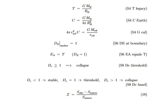
The gravity appendix uses the familiar GM/r reference to connect the RSI scale with its gravity reporting convention. As written, GM/r has specific-energy units, J/kg.

Conditions and scope. This T belongs to the appendix’s stated reference-mass normalization. It cannot be inserted unconverted as a joule quantity in another account. The formula calibrates a mapping; it does not independently determine G without a reference.

LaTeX transcription

T=\frac{G M_\oplus}{R_\oplus}

Source. R2: §15.5; Appendix A.2, A.5

S4 C Earth · eq:S4.CEarth

Earth Carrier Coefficient

C=\frac{G M_\oplus}{4\pi R_\oplus^3}

Read as: C = (G * M_earth) / (4 * pi * R_earth^3)

Equating the Earth carrier–tension tie with the stated GM/r reference yields this coefficient. The same chosen calibration is then available for reuse.

Conditions and scope. In this specific-energy convention C has units J/(kg m²), equivalently s⁻². The energy-ledger coefficient has a different dimensional normalization; the two must not be silently combined.

LaTeX transcription

C=\frac{G M_\oplus}{4\pi R_\oplus^3}

Source. R2: §15.5; Appendix A.5

S4 G cal · eq:S4.Gcal

General Gravity Calibration Relation

4\pi r_{\mathrm{ref}}^2 C=\frac{G M_{\mathrm{ref}}}{r_{\mathrm{ref}}}

Read as: 4 * pi * r_ref^2 * C = G * M_ref / r_ref

This relation states the same calibration tie for a declared reference mass and radius. It identifies which mapping must be held fixed when the result is reused.

Conditions and scope. The explicit radius expression is the evaluated carrier mapping, not an extra factor appended to Equation 1. Reusing a calibration and checking its predictions are separate from fitting a new coefficient for each case.

LaTeX transcription

4\pi r_{\mathrm{ref}}^2 C=\frac{G M_{\mathrm{ref}}}{r_{\mathrm{ref}}}

Source. R2: §15.5; Appendix A.5

D. Section 6 · Boundary identities

These are the one-layer boundary checks and per-layer identity used to keep the field and anchor quantities consistent.

S6 DE at boundary · eq:S6.DEatBoundary

Anchor-Boundary Depth

\left.D_E\right|_{\mathrm{anchor}}=1

Read as: D_E at the anchor boundary = 1

I state the one-layer boundary convention explicitly. It identifies the boundary at which the anchor identity check is applied.

Conditions and scope. An effective depth for a whole multi-anchor system is a different readout. The boundary condition must not be generalized to every system account.

LaTeX transcription

\left.D_E\right|_{\mathrm{anchor}}=1

Source. R2: §15.5, p. 248; Appendix A.3

S6 EA equals T · eq:S6.EAequalsT

Boundary Anchor–Tension Identity

E_A=T\quad(D_E=1)

Read as: E_A = T when D_E = 1

This repeats the boundary identity in the Section 6 family. Its source label remains useful when following an argument that cites that family.

Conditions and scope. The matching field budget and layer convention are retained. A repeated identity is not a new independent premise.

LaTeX transcription

E_A=T\quad(D_E=1)

Source. R2: §15.5; Appendix A.3

S6 T field identity · eq:S6.TfieldIdentity

Per-Layer Tension from the Field Budget

T=\frac{E_F}{D_E}

Read as: T = E_F / D_E

I recover the per-layer budget by dividing the field quantity by the declared nonzero depth. This is Equation 2 rearranged for T.

Conditions and scope. Its interpretation remains energy per participating layer, not ordinary mechanical force or a distance-decaying tension.

LaTeX transcription

T=\frac{E_F}{D_E}

Source. R2: §2.4; Appendix A.3

E. Section 7 · Composite and transfer ledgers

Independent component ledgers, shared-field ledgers, and transfers across a boundary are different accounting choices. I state which account a sum belongs to rather than count the same contribution twice.

S7 composite sum · eq:S7.SigEComposite

Composite Ledger Sum

\Sigma E^{\mathrm{total}}=\sum_i\Sigma E^{(i)}

Read as: SigmaE_total = sum_i(SigmaE_i)

I form a total from the declared component ledgers. The component superscripts identify accounts rather than powers.

Conditions and scope. The accounting convention must prevent double counting a shared interaction. A shared field plus several anchor terms is separately represented by the multi-anchor ledger entry.

LaTeX transcription

\Sigma E^{\mathrm{total}}=\sum_i\Sigma E^{(i)}

Source. R3: “Equation 4: Total Recursive Energy,” pp. 53–55 · R1: §2.4

S7 transfer closed · eq:S7.TransferClosed

Closed-System Transfer

\Delta\Sigma E=\Delta E_F+\Delta E_A=0

Read as: Delta(SigmaE) = Delta(E_F) + Delta(E_A) = 0, for a closed system

This relation states conservation across a transfer within the declared closed boundary. The field and anchor partitions may change while the total remains fixed.

Conditions and scope. An open-system transfer needs its boundary exchange recorded. Setting a change to zero is not justified merely because the variables share a ledger name.

LaTeX transcription

\Delta\Sigma E=\Delta E_F+\Delta E_A=0

Source. R3: “Equation 4: Total Recursive Energy,” pp. 53–55 · R2: §2.2

F. Section 8 · Change-gate bands

The threshold rule and the three-band classification are retained together. Admission is evaluated first. The band classifies the declared configuration; the channel account determines its transition.

S8 Dc threshold · eq:S8.DcThreshold

Change-Threshold Shorthand

D_c\geq1\Rightarrow\mathrm{collapse}

Read as: D_c >= 1 implies collapse, in the source threshold shorthand

The source uses this compact threshold statement alongside the three-way band classification. Unity marks the boundary at which the ordinary stable classification ends.

Conditions and scope. The band entry distinguishes threshold from above-threshold collapse. The shorthand does not specify an instantaneous explosion or replace the transition path, active channels, and pacing conditions.

LaTeX transcription

D_c\geq1\Rightarrow\mathrm{collapse}

Source. R2: Appendix A.6, p. 264

S8 Dc band · eq:S8.DcBand

Stable, Threshold, and Collapse Bands

D_c<1:\ \mathrm{stable};\quad D_c=1:\ \mathrm{threshold};\quad D_c>1:\ \mathrm{collapse}

Read as: D_c < 1: stable; D_c = 1: threshold; D_c > 1: collapse

I keep the three classifications visible so that threshold is not confused with a fully specified transition. These bands belong to the change gate, after the configuration’s admission question.

Conditions and scope. Feasibility still depends on the simultaneous source equations. Where Equation 3 and Equation 5 use the same nonzero account, D_c = D_E; the listed bands are not proof that every band is attainable for an integer-depth account.

LaTeX transcription

D_c<1:\ \mathrm{stable};\quad D_c=1:\ \mathrm{threshold};\quad D_c>1:\ \mathrm{collapse}

Source. R2: Appendix A.6 · R1: §§2.3, 2.5

G. Section 9 · Engine fixed point

The common-load specialization factors Equation 6 before closing Equation 7. Its algebraic consistency condition is distinct from the convergence of a numerical iteration.

S9 Dc fixed point · eq:S9.Dc.fixedpoint

Engine Fixed-Point Relation

D_c^2=\frac{E_F}{K_0 B_T}

Read as: D_c^2 = E_F / (K_0 * B_T)

Under a common load factor, define K_0 as the channel sum without D_c. Then K = K_0 D_c, and substitution into Equation 7 gives the squared-ratio condition.

Conditions and scope. The denominator must be nonzero. A positive real branch requires a positive right-hand side. This algebraic fixed point does not by itself establish that an iterative solver converges to it or that the physical configuration is stable.

LaTeX transcription

D_c^2=\frac{E_F}{K_0 B_T}

Source. R3: “Equation 6: Recursive Engine,” p. 60 · R1: §2.7

H. Section 17 · Transverse contrast

This helper expresses a local transverse contrast in the resolution readout. It belongs to the optical reporting layer.

S17 Z perp · eq:S17.Zperp

Transverse Resolution Contrast

Z_\perp\equiv\frac{\partial_\perp S}{S}\,\delta b

Read as: Z_perp = (partial_perp(S) / S) * delta_b

This local optical helper describes the first-order resolution contrast across a small transverse separation δb. It is the wavefront-imbalance quantity used before a path-integrated readout.

Conditions and scope. The derivative needs a declared differentiable overlay and nonzero S. The product is dimensionless when derivative and separation use compatible length units. It is not the full deflection angle by itself.

LaTeX transcription

Z_\perp\equiv\frac{\partial_\perp S}{S}\,\delta b

Source. R3: “Lensing from RSU Wavefront Imbalance,” pp. 112–114

I. Section 18 · Redshift and composition

I keep the exact source–observer ratio and finite composition law separate from the small-shift approximation, smooth path representation, and separately normalized tension helper.

18 · eq:18-redshift

Explicit Source–Observer Redshift

Z=\frac{S_{\mathrm{obs}}-S_{\mathrm{source}}}{S_{\mathrm{source}}}

Read as: Z = (S_obs - S_source) / S_source

I make the reference in Equation 9 explicit: the source supplies the denominator, and the observer is compared with it. The corresponding ratio is 1 + Z = S_obs/S_source.

Conditions and scope. S_source must be nonzero. Positive Z means S_obs exceeds S_source in this sign convention. A source-frame helper with a different normalization is not silently substituted for this diagnostic.

LaTeX transcription

Z=\frac{S_{\mathrm{obs}}-S_{\mathrm{source}}}{S_{\mathrm{source}}}

Source. R2: Appendix A.10, p. 272 · R3: “Redshift as Structural Collapse,” p. 120

S18 delta k · eq:S18.deltaK

Segment Resolution Shift

\delta_k\equiv\left[\frac{\Delta S}{S}\right]_k

Read as: delta_k = [Delta(S) / S] on segment k

I evaluate each segment relative to its own stated starting readout. The subscript k labels the segment; it is not the engine K.

Conditions and scope. The segment endpoints and reference convention must be compatible for composition. A list of unrelated fractional changes cannot automatically be multiplied into one continuous path ratio.

LaTeX transcription

\delta_k\equiv\left[\frac{\Delta S}{S}\right]_k

Source. R3: “Redshift as Structural Collapse,” p. 121

S18 Z shell sum · eq:S18.Zsum

Small-Shift Sum

Z\approx\sum_k\delta_k

Read as: Z ≈ sum_k(delta_k), in the small-total-correction approximation

The first-order expansion of the composed ratio gives the source’s small-shift sum. It is useful when the omitted products of segment shifts are negligible.

Conditions and scope. Each individual shift being small is not enough for an arbitrarily long path. I also need the accumulated higher-order terms to stay negligible; otherwise I use the finite product rather than the linear sum.

LaTeX transcription

Z\approx\sum_k\delta_k

Source. R3: “Redshift as Structural Collapse,” pp. 121–122; composition statement p. 132

S18 Z composition · eq:S18.Zcomp

Finite Shift Composition

1+Z_{\mathrm{tot}}=\prod_k(1+Z_k)

Read as: 1 + Z_total = product_k(1 + Z_k)

For compatible sequential endpoint ratios, multiplication carries the comparison across the full chain. The intermediate readouts cancel, leaving the final readout divided by the initial one.

Conditions and scope. This is a finite composition rule, not evidence for an actually infinite chain. Nonzero intermediate references and compatible normalization are required.

LaTeX transcription

1+Z_{\mathrm{tot}}=\prod_k(1+Z_k)

Source. R3: “Equation 9: Redshift,” p. 82; “Elios & Tripp Scales,” p. 132

S18 Z continuum · eq:S18.Zcont

Smooth Path Representation

1+Z_{\mathrm{tot}}=\exp\!\left(\int\partial_s\ln S\,ds\right)

Read as: 1 + Z_total = exp(integral(partial_s ln(S) ds))

This is the smooth representation of the sequential ratio when the chosen S is positive and differentiable along the declared path. The parameter s labels that path in the reporting description.

Conditions and scope. I keep the continuum expression as an overlay or limiting representation. Its use does not establish a physically completed infinity of recursion layers or turn s into the primitive depth D_E.

LaTeX transcription

1+Z_{\mathrm{tot}}=\exp\!\left(\int\partial_s\ln S\,ds\right)

Source. R3: “Elios & Tripp Scales,” p. 132

S18 Zt helper · eq:S18.Zt

Tension-Based Shift Helper

Z_t=\frac{E_F D_c}{\theta S_{\mathrm{source}}}

Read as: Z_t = (E_F * D_c) / (theta * S_source), with explicit normalization required

The source records this as a tension-based, non-core helper. It retains its own symbol Z_t and its source-frame state rather than replacing the canonical fractional shift Z.

Conditions and scope. With E_F in energy units and the denominator dimensionless, the displayed quotient still carries energy units. A declared normalization is required before it can represent a dimensionless shift. θ and S_source must be nonzero.

LaTeX transcription

Z_t=\frac{E_F D_c}{\theta S_{\mathrm{source}}}

Source. R1: §2.9 supplement, p. 6 · R3: “Redshift as Structural Collapse,” p. 120

J. Section 19 · Nuclear shell readout

The shell index identifies a particular use of Equation 11. It does not turn the indexed quantities into powers.

S19 NC k · eq:S19.NCk

Nuclear Coupling by Shell

N_C^{k}=\frac{E_A^{k}D_E^{k}}{R_k^2}

Read as: N_C[k] = E_A[k] * D_E[k] / R_k^2

I apply Equation 11 to a declared shell or component k. The superscripts are labels for the component quantities, not exponentiation.

Conditions and scope. Each component must retain a stated budget, separation, and normalization. This indexed relation alone does not prove a nuclear spectrum or select every admissible radius.

LaTeX transcription

N_C^{k}=\frac{E_A^{k}D_E^{k}}{R_k^2}

Source. R3: “Strong and Weak: Closure Notes and Nuclear Radius Ladder,” p. 125

K. Section 20 · Bounds, pacing, and nucleation

The floor convention, optical readout, and common-load nucleation specialization have different jobs. Their shared notation does not remove their stated premises.

S20 Elios axiom · eq:S20.EliosAxiom

Elios Interface Normalization

S(A_{P,\min})=1

Read as: S(A_P_min) = 1

This source notation evaluates the admission ratio at the declared minimum resolved interface and fixes it to unity. It identifies the normalization of the lower-bound discussion.

Conditions and scope. The expression does not supply a measured universal minimum length. It is an interface-domain statement; the later Introduction distinguishes the end of a resolved external description from a claim that nothing exists beyond it.

LaTeX transcription

S(A_{P,\min})=1

Source. R3: “Elios & Tripp Scales,” pp. 127–131 · R2: §13.2, pp. 208–209

S20 Z frame ratio · eq:S20.ZframeRatio

Emission–Observation Frame Ratio

1+Z=\frac{S_{\mathrm{obs}}}{S_{\mathrm{emit}}}

Read as: 1 + Z = S_obs / S_emit

This is Equation 9 written as a ratio between the emitted and observed resolution readouts. It keeps the source convention explicit in the scale discussion.

Conditions and scope. The two readouts need compatible normalization and S_emit ≠ 0. A large ratio is not, by itself, an independently established clock, lensing, or cosmological law.

LaTeX transcription

1+Z=\frac{S_{\mathrm{obs}}}{S_{\mathrm{emit}}}

Source. R3: “Elios & Tripp Scales,” p. 129 · R2: Appendix A.8.1

S20 alpha grad · eq:S20.alphaGrad

Path-Integrated Deflection Helper

\alpha(b)\approx\int\partial_\perp\ln S\,ds

Read as: alpha(b) ≈ integral(partial_perp ln(S) ds)

I represent optical bending through the accumulated transverse logarithmic contrast along a declared ray path. The impact parameter b identifies the path family.

Conditions and scope. α(b) is an angle-like overlay readout, not the strong coupling α_RSI or the allocation scale α_Q. The approximation needs a specified positive S field, path, and observational mapping; it is not a complete lensing solution without them.

LaTeX transcription

\alpha(b)\approx\int\partial_\perp\ln S\,ds

Source. R3: “Elios & Tripp Scales,” p. 132 · R2: §8.10; Appendix A.8.1

S20 K linear · eq:S20.Klin

Common-Load Engine Factorization

K=K_0 D_c

Read as: K = K_0 * D_c

For a common D_c, I can factor that load out of Equation 6 and define K_0 = sum(K_ch θ). The equation is the linear engine assumption used in the fixed-point and nucleation calculations.

Conditions and scope. It does not follow in this form for independently varying channel loads unless an additional effective definition is supplied. K_0 remains the declared channel sum, not the admission gate.

LaTeX transcription

K=K_0 D_c

Source. R3: “Equation 6: Recursive Engine,” p. 60; “Engine–nucleation scaffold,” p. 132

S20 Sigma QTheta · eq:S20.SigmaQTheta

Orientation-Weighted Partner Sum

\Sigma_{Q\theta}\equiv\sum_i(Q_i\theta_i)

Read as: Sigma_Qtheta = sum_i(Q_i * theta_i)

I collect the partner contributions with their orientation factors before multiplying by the common collapse ratio used in the nucleation specialization. It is a partner sum, distinct from the channel sum K_0.

Conditions and scope. The fixed-point specialization assumes a common D_c and the same declared anchor budget. A negative or cancelling sum does not automatically provide a positive energy branch.

LaTeX transcription

\Sigma_{Q\theta}\equiv\sum_i(Q_i\theta_i)

Source. R3: “Engine–nucleation scaffold,” Theorem 19.6, pp. 132–133

S20 nucleation tri · eq:S20.NucleationTri

Nucleation Tri-Identity

E_A^*=\sqrt{E_F\Sigma_{Q\theta}}=\sqrt{E_F K_0 B_T},\quad\Sigma_{Q\theta}=K_0 B_T

Read as: E_A_star = sqrt(E_F * Sigma_Qtheta) = sqrt(E_F * K_0 * B_T); Sigma_Qtheta = K_0 * B_T

With a common D_c, Equation 10 gives E_A = D_c Σ_Qtheta. Combining this with Equation 5 gives E_A² = E_F Σ_Qtheta. The common-load engine closure then supplies the matching condition Σ_Qtheta = K_0 B_T.

Conditions and scope. The positive-root expression requires the positive, nonzero branch assumed by the calculation. It remains a conditional closure identity. It does not establish that a cosmological nucleation occurred or provide an unaccounted source of energy.

LaTeX transcription

E_A^*=\sqrt{E_F\Sigma_{Q\theta}}=\sqrt{E_F K_0 B_T},\quad\Sigma_{Q\theta}=K_0 B_T

Source. R3: “Engine–nucleation scaffold,” Theorem 19.6, pp. 132–133

S20 BT req · eq:S20.BTreq

Boundary Term Required by the Match

B_{T,\mathrm{req}}=\frac{\Sigma_{Q\theta}^{\mathrm{given}}}{K_0}

Read as: B_T_required = Sigma_Qtheta_given / K_0

I solve the tri-identity’s coefficient match for B_T while holding the given partner sum and channel coefficient fixed. This states the value required by that equality.

Conditions and scope. K_0 must be nonzero and the result must be compatible with the chosen branch and units. A claim that it is a physical minimum needs the accompanying threshold or ordering conditions, not this division alone.

LaTeX transcription

B_{T,\mathrm{req}}=\frac{\Sigma_{Q\theta}^{\mathrm{given}}}{K_0}

Source. R3: “Engine–nucleation scaffold,” Corollary 19.7, p. 133

S20 alpha Q · eq:S20.alphaQ

Partner-Sum Matching Scale

\alpha_Q=\frac{K_0B_T}{\Sigma_{Q\theta}^{\mathrm{given}}}

Read as: alpha_Q = (K_0 * B_T) / Sigma_Qtheta_given

This quotient gives the scale that would bring a stated partner sum into the same fixed-point coefficient match. It is a derived comparison of the declared quantities.

Conditions and scope. The given partner sum must be nonzero. α_Q is neither a strong coupling nor an optical deflection angle, and it is not permission to adjust partner budgets after a failed empirical prediction without declaring the change.

LaTeX transcription

\alpha_Q=\frac{K_0B_T}{\Sigma_{Q\theta}^{\mathrm{given}}}

Source. R3: “Engine–nucleation scaffold,” Corollary 19.7, p. 133

L. Section 21 · Exterior horizon helpers

These expressions are evaluated in a declared exterior accounting. The boundary of that accounting is not an assertion that an unresolved interior does not exist.

S21 · eq:S21.horizon

Last-Resolved Horizon Condition

S(r_h)=\frac{E_A}{A_P(r_h)}=1

Read as: S(r_h) = E_A / A_P(r_h) = 1

I identify a last resolved shell in a declared exterior accounting through its admission condition. The relevant carrier is evaluated at the horizon radius r_h.

Conditions and scope. A horizon in this account is not a point singularity or a declaration that the interior does not exist. The exterior context and the domain of the carrier have to be specified.

LaTeX transcription

S(r_h)=\frac{E_A}{A_P(r_h)}=1

Source. R2: §13.3, p. 210 · R3: “Time-Dilation at the Tripp Scale; Black-Shell Horizons and Interiors,” p. 134

S21 · eq:S21.Zext

Exterior Reference Shift

Z_{\mathrm{ext}}=\frac{S_{\mathrm{ref}}-S(r)}{S(r)}\quad(r>r_h)

Read as: Z_ext = (S_ref - S(r)) / S(r), for r > r_h

I compare the local exterior resolution readout with the declared reference. The condition r > r_h keeps the stated application on the exterior side of the horizon.

Conditions and scope. S(r) must be nonzero and the reference normalization must remain fixed. This diagnostic does not justify extending the exterior calculation through an unresolved interior.

LaTeX transcription

Z_{\mathrm{ext}}=\frac{S_{\mathrm{ref}}-S(r)}{S(r)}\quad(r>r_h)

Source. R3: “Time-Dilation at the Tripp Scale; Black-Shell Horizons and Interiors,” pp. 134–135 · R2: §13.3

M. Further source relations

The following relations retain their own source roles: a shared-field ledger, normalized readouts, two explicitly non-core supplements, and the depth-resolved bridge. They do not extend the Core-12 numbering.

Multi-ledger · source-specific relation

Shared-Field Multi-Anchor Ledger

\Sigma E_R=E_F+\sum_j E_{A,j}

Read as: SigmaE_R = E_F + sum_j(E_A_j)

The Core-12 reference separately gives this shared-field ledger convention for several anchors. The field term appears once and the declared anchor contributions are added explicitly.

Conditions and scope. This convention differs from summing independent component ledgers. The chosen accounts must make shared energy and boundary exchanges explicit.

LaTeX transcription

\Sigma E_R=E_F+\sum_j E_{A,j}

Source. R1: §2.4, p. 4

P4 ledger share · source-specific relation

f_i=\frac{Q_i\theta_i D_{c,i}}{\sum_j(Q_j\theta_j D_{c,j})}

Read as: f_i = (Q_i * theta_i * D_c_i) / sum_j(Q_j * theta_j * D_c_j)

I normalize the contributions already present in Equation 10. For a nonzero denominator, the shares sum to one. The normalization reports how the declared partner sum is distributed; it does not replace that sum.

Conditions and scope. Signed contributions can produce negative shares or shares above one. Summing to one alone does not make them probabilities or nonnegative membership weights.

LaTeX transcription

f_i=\frac{Q_i\theta_i D_{c,i}}{\sum_j(Q_j\theta_j D_{c,j})}

Source. R2: §4.8; Appendix A.8, p. 266

Overview allocation · source-specific relation

Normalized Stability-Influence Allocation

\lambda_{ij}=\frac{E_{A,i}/A_{P,i}}{\sum_k(E_{A,k}/A_{P,k})}

Read as: lambda_ij = (E_A_i / A_P_i) / sum_k(E_A_k / A_P_k)

The Introduction’s one-page overview displays this allocation diagnostic under its Equation 10 heading. It normalizes stability-like contributions, while the detailed solver summary and Appendix A.8 identify Equation 10 as the partner-budget sum.

Conditions and scope. I keep the expressions separate. Their inputs and output roles differ, so one cannot be substituted for the other merely because a heading number matches. The index roles and nonzero denominator must be declared for the application.

LaTeX transcription

\lambda_{ij}=\frac{E_{A,i}/A_{P,i}}{\sum_k(E_{A,k}/A_{P,k})}

Source. R2: §1.9, p. 33; §15.5, p. 247; Appendix A.8

Overview weak diagnostic · source-specific relation

Weak Threshold-Excess Diagnostic

W_c=D_c-1

Read as: W_c = D_c - 1

The one-page overview places this dimensionless threshold excess under its Equation 12 heading. It reports the difference from unity; it does not add a new independent physical quantity.

Conditions and scope. The procedural weak-closure statement remains the Core-12 reference form. W_c is not a decay rate, lifetime, or a completed channel mechanism.

LaTeX transcription

W_c=D_c-1

Source. R2: §1.9, p. 34; §15.5, p. 247

8f · source-specific relation

Laplacian Modeling Supplement

\nabla^2 E_A=D_E\sum_i U_i

Read as: Laplacian(E_A) = D_E * sum_i(U_i)

The Core-12 reference explicitly labels this a modeling supplement for gradient or curvature work. The scalar counting form remains Equation 8.

Conditions and scope. The operator, coordinates, source interpretation, and unit mapping have to be supplied. With ordinary length coordinates, applying a Laplacian changes the left-hand units, so the supplement cannot be treated as dimensionally identical to the counting equation without further declarations.

LaTeX transcription

\nabla^2 E_A=D_E\sum_i U_i

Source. R1: §2.8 supplement, p. 5

R0-D depth · source-specific relation

Effective System Depth

D_{E,\mathcal S}^{\mathrm{eff}}=\frac{\sum_j(Q_j\theta_jD_{c,j})}{\sum_i U_i}

Read as: D_E_eff(system) = sum_j(Q_j * theta_j * D_c_j) / sum_i(U_i)

The depth-resolved result applies the identity tally and partner closure to the same declared anchor budget. Equating those accounts and dividing by the nonzero identity tally gives this effective depth.

Conditions and scope. The system, identities, carrier, normalization, and shared-budget condition are premises. The readout does not turn D_E into a radial coordinate or establish that an arbitrary effective value is a primitive integer-layer count.

LaTeX transcription

D_{E,\mathcal S}^{\mathrm{eff}}=\frac{\sum_j(Q_j\theta_jD_{c,j})}{\sum_i U_i}

Source. R2: Appendix A.8.1, Theorem A.7, pp. 267–268 · R4: Appendix A, Proposition A.68

R0-D state · source-specific relation

Depth-Resolved Admission Readout

S_{\mathcal S}=\frac{D_{E,\mathcal S}^{\mathrm{eff}}\sum_i U_i}{A_P(\mathcal S)}

Read as: S_system = D_E_eff(system) * sum_i(U_i) / A_P(system)

I substitute the shared-budget depth expression into Equation 1. The system’s identity inventory remains in the numerator and the declared carrier remains in the denominator.

Conditions and scope. The resulting S is still an admission readout. Geometry belongs to A_P(system); it cannot be discarded and replaced by an unqualified depth-only law.

LaTeX transcription

S_{\mathcal S}=\frac{D_{E,\mathcal S}^{\mathrm{eff}}\sum_i U_i}{A_P(\mathcal S)}

Source. R2: Appendix A.8.1, pp. 267–269 · R4: Appendix A, Proposition A.68

R0-D full ratio · source-specific relation

Full Depth–Inventory–Carrier Contrast

1+Z=\frac{D_{E,\mathrm{obs}}^{\mathrm{eff}}\sum_i U_{i,\mathrm{obs}}}{D_{E,\mathrm{emit}}^{\mathrm{eff}}\sum_i U_{i,\mathrm{emit}}}\frac{A_{P,\mathrm{emit}}}{A_{P,\mathrm{obs}}}

Read as: 1 + Z = [D_E_eff_obs * sum_i(U_i_obs)] / [D_E_eff_emit * sum_i(U_i_emit)] * A_P_emit / A_P_obs

The full comparison retains three possible sources of contrast: effective depth, participating identity inventory, and the carrier. It follows by substituting the depth-resolved admission readout into the source–observer ratio.

Conditions and scope. The denominators must be nonzero and the compared accounts compatible. Reading the contrast as clock pacing, redshift, or a path delay requires the specific observational mapping and its evidence.

LaTeX transcription

1+Z=\frac{D_{E,\mathrm{obs}}^{\mathrm{eff}}\sum_i U_{i,\mathrm{obs}}}{D_{E,\mathrm{emit}}^{\mathrm{eff}}\sum_i U_{i,\mathrm{emit}}}\frac{A_{P,\mathrm{emit}}}{A_{P,\mathrm{obs}}}

Source. R2: Appendix A.8.1, pp. 268–269 · R4: Appendix A, Proposition A.68 and Theorem A.69

R0-D controlled ratio · source-specific relation

Controlled Depth-Ratio Approximation

1+Z\approx\frac{D_{E,\mathrm{obs}}^{\mathrm{eff}}}{D_{E,\mathrm{emit}}^{\mathrm{eff}}}

Read as: 1 + Z ≈ D_E_eff_obs / D_E_eff_emit, under controlled inventory and carrier conditions

The source gives this restricted comparison when the identity inventory and relevant carrier contribution are controlled so that the other factors in the full expression cancel or are appropriately approximated.

Conditions and scope. Holding a carrier coefficient fixed does not automatically make two carrier values equal. The full ratio remains the governing expression unless those factors are controlled. The internal result is not independent confirmation of every timing or lensing dataset.

LaTeX transcription

1+Z\approx\frac{D_{E,\mathrm{obs}}^{\mathrm{eff}}}{D_{E,\mathrm{emit}}^{\mathrm{eff}}}

Source. R2: Appendix A.8.1, Corollary A.9 and claim-tier note, p. 269 · R4: Appendix A, Proposition A.68 and Theorem A.69

Sources and locations

I identify the source and its local role rather than treat every edition, overview, or supplement as one interchangeable formula list. Page numbers below refer to the named source text. Publication links lead to the related reading page; they are not PDF page links.

R1 · RSI / DRRSUI Core-12 reference
Matthew Tripp Zejda. The compact seven-page Core-12 reference: §2 gives the twelve reference forms; §§2.8–2.12 identify the modeling supplement, tension helper, partner closure, and procedural weak-domain statement. The source’s geometry restriction keeps distance in A_P and the declared strong-domain exception.
RSI publication and reading access
R2 · Resolution State Interface: Introduction to Universal Relativity
Matthew Tripp Zejda. The 428-page Introduction reference. Principal locations: §1.9, pp. 30–34; §1.20.5, pp. 40–42; §2.4, pp. 51–55; §4.8, pp. 81–82; §7.4, pp. 118–123; §13.3, pp. 210–211; §15.5, pp. 246–248; Appendix A, pp. 255–273; Appendices E–F, pp. 312–323. R0-D is Theorem A.7 in §A.8.1, with its controlled comparisons and claim boundaries.
Introduction to Universal Relativity
R3 · Extended RSI equation treatments
Matthew Tripp Zejda. The extended 360-page RSI treatment: “Equation 6: Recursive Engine,” pp. 60–63; “Equation 11: Nuclear Coupling,” pp. 91–93; “Lensing from RSU Wavefront Imbalance,” pp. 112–117; “Redshift as Structural Collapse,” pp. 118–122; nuclear shell readouts, pp. 125–126; “Elios & Tripp Scales” and the engine–nucleation results, pp. 127–133; exterior horizon readouts, pp. 134–135. These locations supply the older named helper families, not a replacement for the later Introduction’s role and normalization distinctions.
Related RSI publication
R4 · Existential Ground
Matthew Tripp Zejda. Chapter 13, “RSI as the Physical Bridge”; Appendix A, Proposition A.68, “Depth-Resolved Pacing Bridge, Conditional Form,” and Theorem A.69, “RSI Physical-Bridge Conditionality.” The logical account specifies burdens for a physical implementation; it does not certify its coefficients, carriers, or empirical predictions by itself.
Existential Ground

A

B

C

D

E

F

G

H

I

K

L

M

N

O

P

Q

R

S

Symbols

T

U

W

Z

Reading the equations

Keep the account and its units fixed

A. Core-12

Resolution State Law

Recursive Field Energy

Anchor Energy

Total Recursive Energy

Deterministic Collapse Ratio

Recursive Engine

Engine-Regulated Closure

Identity Summation

Recursive Redshift

Multi-Body Anchor Closure

Nuclear Coupling

Weak-Domain Closure

B. Strong-domain helpers · S11

Strong-Domain Resolution Scale

Dimensionless Strong Coupling

Coupling Form of Nuclear Normalization

Logarithmic Coupling Model

Beta Function of the Logarithmic Model

Two-Point Calibration of b

Planar-to-Line Tension Readout

Strong-Domain Matching Condition

Fixed Point with a Local Channel Sum

Finite-Window Power-Law Coupling

C. Section 4 · Interface and calibration

Section 4 Admission Definition

Section 4 Ledger Definition

Section 4 Shift Definition

Spherical Anchor-Plane Carrier

One-Layer Field Budget

One-Layer Anchor Budget

Earth Reference Carrier

Earth Admission Pin

Earth Carrier–Tension Tie

Gravity Reference in Specific-Energy Units

Earth Carrier Coefficient

General Gravity Calibration Relation

D. Section 6 · Boundary identities

Anchor-Boundary Depth

Boundary Anchor–Tension Identity

Per-Layer Tension from the Field Budget

E. Section 7 · Composite and transfer ledgers

Composite Ledger Sum

Closed-System Transfer

F. Section 8 · Change-gate bands

Change-Threshold Shorthand

Stable, Threshold, and Collapse Bands

G. Section 9 · Engine fixed point

Engine Fixed-Point Relation

H. Section 17 · Transverse contrast

Transverse Resolution Contrast

I. Section 18 · Redshift and composition

Explicit Source–Observer Redshift

Segment Resolution Shift

Small-Shift Sum